Electrostatic Interactions
Overview
Teaching: 10 min
Exercises: 0 minQuestions
How electrostatic interactions are calculated in periodic systems?
Objectives
Learn what parameters control the accuracy of electrostatic calculations
Coulomb interactions
- Long range: $V_{Elec}=\frac{q_{i}q_{j}}{4\pi\epsilon_{0}\epsilon_{r}r_{ij}}$
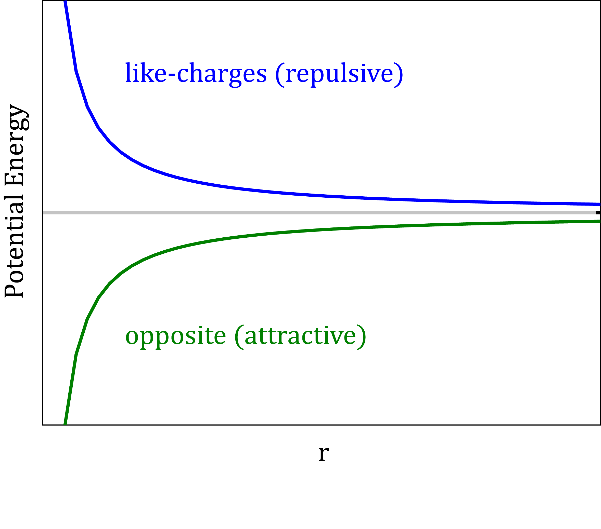
Electrostatic interactions decay slowly with distance. An electrostatic interaction calculation must include particles within at least 100 A for reasonable accuracy. Due to this long-range behavior, the task of computing Coulomb potentials is often the most time consuming part of any MD simulation. Computing electrostatic energy by direct summation of all pairwise interactions would be prohibitively slow even in a system without periodic boundary condition. To complicate things in periodic systems it is necessary to compute contributions from all periodic images (lattice sum). To accelerate these calculations, fast and efficient algorithms are needed.
- Computing Coulomb potentials is often the most time consuming part of any MD simulation.
- Fast and efficient algorithms are required for these calculations.
Particle Mesh Ewald (PME)
Particle Mesh Ewald (PME) method is the most widely used method using the Ewald decomposition technique. The potential is decomposed into two parts: a fast decaying and a slow decaying. A fast decaying part is computed in real space. A slow decaying part is computed in Fourier space (reciprocal space).
- The most widely used method using the Ewald decomposition.
- The potential is decomposed into two parts: fast decaying and slow decaying.

Fast decaying short-ranged potential (Particle part).
The real space sum is short-ranged and as for the LJ potentials, it can be truncated when sufficiently decayed. It is a direct sum of contributions from all particles within a cutoff radius. It is the Particle part of PME.
- Sum of all pairwise Coulomb interactions within a cutoff radius
- Implements same truncation scheme as the LJ potentials.
Slow decaying long-ranged potential (Mesh part).
The Fourier space part, on the other hand, is long-ranged but smooth and periodic. This part is a slowly varying function. PME takes advantage of the fact that all periodic functions can be represented with a sum of sine or cosine components, and slowly varying functions can be accurately described by only a limited number of low frequency components (k vectors). In other words Fourier transform of the long-range Coulomb interaction decays rapidly in Fourier space, and summation converges fast.
- Slowly varying, smooth and periodic function.
- All periodic functions can be represented with a sum of sine or cosine components.
- Slowly varying functions can be accurately described by only a limited number of low frequency components (k vectors).
PME algorithm
The long range contribution can then be efficiently computed in Fourier space using FFT. Fourier transform calculation is discrete and requires the input data to be on a regular grid. It is the Mesh part of PME. As point charges in a simulation are non-equispaced, they need to be interpolated to obtain charge values in equispaced grid cells.
- Long-range electrostatic interactions are evaluated using 3-D grids in reciprocal Fourier space.
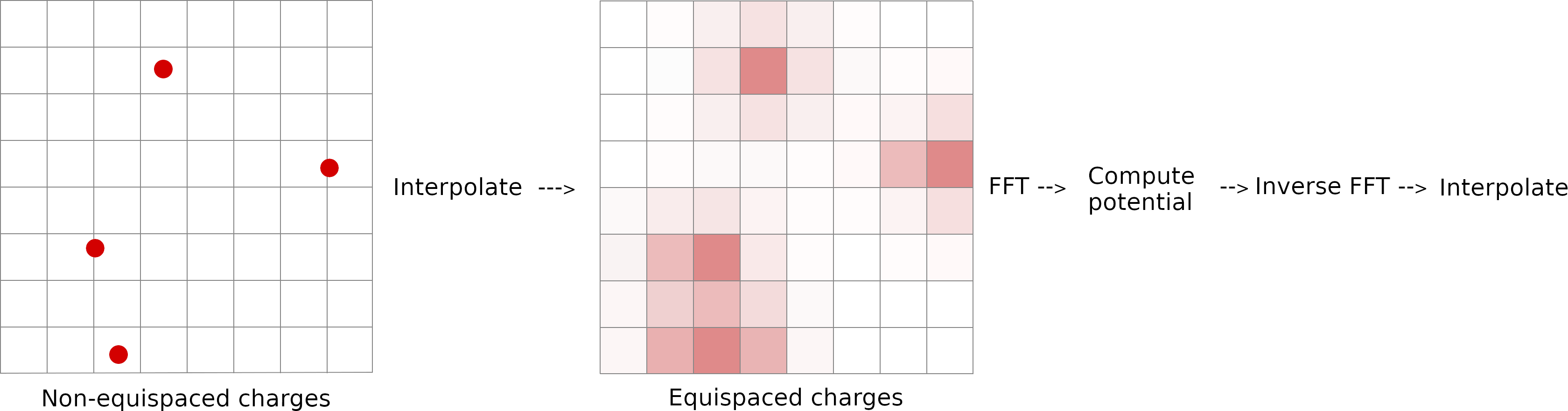
- The first step of PME calculation is to assign charges to grid cells. Charges in the grid cells are obtained by interpolation.
- After interpolation discrete Fourier transform is computed.
- Then potential in grid cells is calculated. Coulomb interaction decays rapidly in Fourier space, and summation converges fast.
- Inverse Fourier transform is computed to transform gridded potentials to real space.
- Finally gridded potentials are interpolated back to atomic centers.
Simulation parameters controlling speed and accuracy of PME calculations.
Having learned how electrostatic potential is calculated, we can now examine the parameters controlling speed and accuracy of PME calculations.
-
Grid spacing and dimension. Grid dimension values give the size of the charge grid in each dimension. Higher values lead to higher accuracy but considerably slow down the calculation. Generally it has been found that reasonable results are obtained when grid dimension values are approximately equal to periodic box size, leading to a grid spacing of 1.0 Å. Significant performance enhancement in the calculation of the fast Fourier transform is obtained by having each of the values be a product of powers of 2, 3, and/or 5. If the values are not given, programs will chose values to meet these criteria.
-
Direct space tolerance. Controls the splitting into direct and reciprocal part. Higher tolerance shifts more charges into Fourier space.
-
Interpolation order is the order of the B-spline interpolation. The higher the order, the better the accuracy (unless the charge grid is too coarse). The minimum order is 3. An order of 4 (the default) implies a cubic spline approximation which is a good standard value.
- Grid spacing. Lower values lead to higher accuracy but considerably slow down the calculation. Default 1.0 Å.
- Grid dimension. Higher values lead to higher accuracy but considerably slow down the calculation.
- Direct space tolerance. Controls the splitting into direct and reciprocal part. Higher tolerance shifts more charges into Fourier space.
- Interpolation order is the order of the B-spline interpolation. The higher the order, the better the accuracy. Default 4 (cubic spline).
Poll 6. Electrostatic interactions
Which of the following statements is incorrect? For more accurate electrostatic calculations you need to:
- Decrease grid spacing
- Increase the grid dimensions
- *Increase direct space tolerance
- Increase the interpolation order
- Higher tolerance shifts more charges into Fourier space and calculations in Fourier space are less accurate than direct summation.
| Variable \ MD package | GROMACS | NAMD | AMBER |
|---|---|---|---|
| Fourier grid spacing | fourierspacing (1.2) | PMEGridSpacing (1.5) | |
| Grid Dimension X | fourier-nx | PMEGridSizeX | nfft1 |
| Grid Dimension Y | fourier-ny | PMEGridSizeY | nfft2 |
| Grid Dimension Z | fourier-nz | PMEGridSizeZ | nfft3 |
| Direct space tolerance | ewald-rtol (\(10^{-5}\)) | PMETolerance (\(10^{-5}\)) | dsum_tol (\(10^{-6}\)) |
| Interpolation order | pme-order (4) | PMEInterpOrder (4) | order (4) |
| Variable \ MD package | GROMACS | NAMD | AMBER |
|---|---|---|---|
| Fourier grid spacing | fourierspacing (1.2) | PMEGridSpacing (1.5) | |
| Grid Dimension [X,Y,Z] | fourier-[nx,ny,nz] | PMEGridSize[X,Y,Z] | nfft[1,2,3] |
| Direct space tolerance | ewald-rtol (\(10^{-5}\)) | PMETolerance (\(10^{-5}\)) | dsum_tol (\(10^{-6}\)) |
| Interpolation order | pme-order (4) | PMEInterpOrder (4) | order (4) |
Key Points
Calculation of electrostatic potentials is the most time consuming part of any MD simulation
Long-range part of electrostatic interactions is calculated by approximating Coulomb potentials on a grid
Denser grid increases accuracy, but significantly slows down simulation